![]() Example
1: Arbitrage Free Price of a Stock Index Future
Example
1: Arbitrage Free Price of a Stock Index Future
The following example first illustrates how the arbitrage free price of a forward contract is identified using the cost of carry model. This is applied to a futures contract by assuming that the impact of marking to market upon the arbitrage free price is zero. This assumption turns out to be reasonable in practice for any short maturity futures including interest rate futures.
The cost of carry approach
to arbitrage free pricing is first applied assuming discrete compounding. We then apply the model assuming continuous
compounding, which is consistent with the FTS Futures Module’s calculator and
is easier to apply to the real world futures markets. Following the examples below we provide an example
of estimating the implied constant continuous dividend yield from an index
future using the futures calculator module.
The S&P500 Index Future trading on the Chicago Mercantile Exchange have a minimum fluctuation equal to 0.05 (5-points). That is, the total minimum fluctuation is $12.50 or $2.5 per point.
Quotation Convention: The price that the index future settles at. This is $250 times the Standard & Poor's 500 Stock Index.
Note: CME also trades a smaller contract referred to as the E-mini S&P500 contract. This is a stock index future that settles at $50 times the Standard & Poor's 500 Stock Index.
S&P 500 Future Example: Suppose the 6-month Index future quotation is 1208.20 and you are long 1 future contract. This means that at the time of settlement you are obligated to pay $250*1208.20 in exchange for receiving $250*S&P 500 Index Number.
Assume that the 6-month risk free rate that can be borrowed or lent at is 3% per annum (compounded semi-annually). Finally, as a simplifying assumption assume that at the end of 6-months a dividend is paid at the rate of 0.65%. Finally, suppose the spot index value is 1197.903.
Valuing the Index Future Using Cost of Carry (Discrete
Compounding)
The Cost of Carry approach to valuing the Index Future identifies the cost of the synthetic equivalent contract. The synthetic equivalent is formed by borrowing cash at 3% for 6-months, buying the underlying index at the spot price and holding this position for 6-months. At the end of 6-months the transactions are reversed so that the underlying index is sold and the loan is repaid.
Synthetic Future
Time t=0
Borrow $250*1197.903 = $299,475.75
Buy 250 “units” of the underlying index at 1197.903 per unit.
Time t=1
Receive $250*$7.69 = $1922.50 in dividends
Sell 500 “units” of the underlying index @ S, this generates +$250*S
Repay loan $299,475.75*(1+0.03/2) = $303,967.89
Note:
Semi-annual compounding is assumed above. The general form if interest is compounded t
times per year and principal P is invested for n years at the discrete rate r/t
period for nt periods then the future value of the
principal after nt periods is P(1+r/t)^(nt).
In the above example n = 0.5 and t=2.
Net Result at time t=1: You own 250 units of the underlying valued at $250*S for a cost of $303,967.89 - $1922.50 = $302045.39
Actual Future (Ignoring Margins)
Time t=0
Buy 1 futures contract at $1208.2, at this time no cash is exchanged.
Time t=1
Receive +$250*S pay $1208.2*250 = $302,050
So with this alternative you have acquired 500 units of the underlying at a cost of $302,050.
Aside: Up to rounding errors the two alternatives are identical. In this example the rounding error is induced by using the risk free rate to 2-decimal places. If you wanted to verify the numbers precisely then try using 3.00308% for the risk free rate in the above example.
Remark: Notice that the dividends paid by the underlying represent a reduction to the cost of borrowing when creating the synthetic equivalent to the futures contract. As a result they represent a reduction in the carry costs.
Valuing the Index Future Using Cost of Carry (Continuous
Compounding)
The Cost of Carry approach to valuing the Index Future identifies the cost of the synthetic equivalent contract. The synthetic equivalent is formed by borrowing cash for 6-months at the continuous compounded rate (= 0.029777) for 6-months, buying the underlying index at the spot price and holding this position for 6-months. At the end of 6-months the transactions are reversed so that the underlying index is sold and the loan is repaid.
Aside: If the compounding frequency is continuous then the continuous compounded rate is r, and if time is n periods then the initial principal grows at the rate of Pexp(rn). If $100 grows at the rate of 0.03/2 for 6-months (i.e., 3% compounded semi annually) and therefore equals $101.50, then the implied continuous compounded rate r that equates the $100 to a future value of $101.50 after 6-months is 0.029777 ($100*exp(0.029777*0.5) = $101.50). The FTS Calculator automates these conversions for you.
Assume further that the constant continuous dividend yield rate for the S&P 500 index is 0.012659.
Synthetic Future
Time t=0
Borrow $250*1197.903 = $299,475.75
Buy 250 “units” of the underlying index at 1197.903 per unit
Time t=1
Sell 250 “units” of the underlying index @ S, this generates +$250*S
Repay loan net of the constant continuous dividend yield received from index $299,475.75*(exp((0.029777- 0.012659)*0.5)) = $302,050
Net Result at time t=1: You own 250 units of the underlying valued at $250*S for a cost of $302,050.
Actual Future (Ignoring Margins)
Time t=0
Buy 1 futures contract at $1208.2, at this time no cash is exchanged.
Time t=1
Receive +$250*S pay $1208.2*250 = $302,050
So with this alternative you have acquired 250 units of the underlying at a cost of $302,050.
The two alternatives are identical.
Backing Out Information from Observed Futures Prices
Suppose you want to know what is the implied dividend yield for the S&P 500 index at a point in time? This information is not usually provided but with a little knowledge about the futures prices you can make a pretty good guess at it assuming the futures prices are arbitrage free.
How?
You can observe both the futures price and the spot S&P500 index prices plus you can infer the interest rate from the yield curve. The only missing piece of information is the dividend yield.
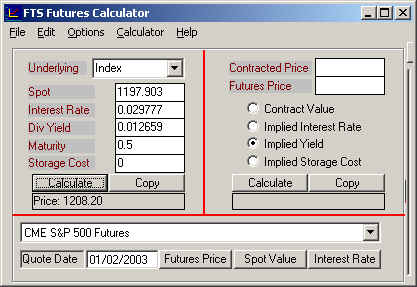
You can now solve for the implied dividend yield from the calculator as follows. If the 6-months futures price is 1208.2 and the interest rate is 0.029777 (continuously compounded) we can verify that the implied constant continuous dividend yield is 0.0127. Enter the numbers into the calculator as displayed below (i.e., enter all numbers into the left side and the futures price into the right hand side):
Now select Implied Yield as above and click on Calculate:
Summary:
Futures prices are useful for making forecasts about the market. Other examples are suppose 30-minutes before the market opens you are asked to forecast whether the opening is likely to be up or down? You can answer this by backing out the implied spot price that supports the current futures price which you can observe hours before the US markets open.
Online you can work through an actual real world example for computing the implied constant dividend yield by clicking on the hypertext Example 2.