
Working with the BDT Model
Introduction
This is a simple but very powerful module. It generates interest rate trees that will let you value any interest rate derivative or sequence of cash flows, that can be represented on the tree. In particular, the module produces risk neutral interest rate trees consistent with two important real world constraints: i. prices are consistent with the current spot yield curve, and ii. prices are consistent with the current volatility structure (volatility as a function of time to maturity).
You can apply the module to your own inputs (i.e., yield curve and volatility structure). The output is designed to be used in conjunction with Excel. That is, the module provides the interest rate tree and the user provides the valuation problem in their spreadsheet. Thus it can be applied to producing valuations that are consistent with information contained in the yield curve, for any instrument.
Motivation for an Interest Rate Tree
In the real world interest rates change over time and exhibit mean reverting behavior. Furthermore, these dynamics have a significant impact upon the price of any interest rate derivative. Therefore, when valuing interest rate derivatives the model used should incorporate, to the extent possible, persistent stylized facts associated with interest rate dynamics.
Black Derman and Toy, developed an algorithmic solution to this problem. The strength of their contribution is that although it is simple to implement it produces prices consistent with prices from other fixed income markets. In particular, the price or present value is consistent with both the current (relevant) spot yield curve and relevant volatility structure.
Whenever, either of these two constraints change then a new price must be estimated.
Example: Constructing and Interpreting an Interest Rate Tree
Suppose the spot yield curve has the following characteristics (the default data in the BDT module):
|
Time to
Maturity |
Spot Rate |
Volatility
of the Log(rate) |
|
1 |
0.10 |
.20 |
|
2 |
0.11 |
.19 |
|
3 |
0.12 |
.18 |
|
4 |
0.13 |
.17 |
|
5 |
0.14 |
.16 |
Can we construct a set of interest rate numbers that satisfy these two constraints?
The answer is yes, and one algorithm for doing so was first supplied by Black Derman and Toy. By using the BDT module we can construct the interest tree consistent with the data above.
Step 1: First, open an Excel spreadsheet and then link the BDT module to this spreadsheet by clicking on the button Find Excel Sheets. Next leave Bond Price Data unchecked and check Local Volatility Data. This means that you are using spot yields to maturity plus the volatlity structure to compute the interest rate tree from. Click on the button "Fit Lattice" and finally, click on the button "Transfer Entire Lattice to Excel."
Note: If you want to start with price data as opposed to yields then you would check price data.
Now you have an interest tree that is consistent with the spot yield curve and the volatility structure for the spot yield curve. It is noted, however, that the interest rate tree is not meant to represent how true rates are likely to be over time. Instead it represents a set of interest rate numbers that produce prices consistent with the two constraints above (spot yields to maturity, and volatilities).
The actual interest rate tree numbers exported to Excel are provided below for the beginning of each year. The risk neutral probability for an up- or down-tick is 0.5 for this tree.
| Year 1 | Year 2 | Year 3 | Year 4 | Year 5 |
| 0.338464 | ||||
| 0.262012 | ||||
| 0.196941 | 0.245776 | |||
| 0.14318 | 0.186493 | |||
| 0.1 | 0.137401 | 0.17847 | ||
| 0.097916 | 0.13274 | |||
| 0.095862 | 0.129596 | |||
| 0.09448 | ||||
| 0.094106 |
Question 1: Does the above tree, produced from the BDT module, satisfy the volatility constraint?
To check this recall that the tree is constructed from the log of the spot rates. As a result, volatility is estimated from the difference of the log rates divided by 2. When viewed from today the beginning of year 1 spot rate is known and so there is zero volatility associated with 0.1. There are, however, two possible year 2 rates. As a result, the volatility is (log(0.14318) - log(0.097916))/2 = 0.19. There are three possible year 3 rates from which any pair of adjacent rates in the tree will give the year three volatility. You can verify that this is 0.18, and so on.
Question 2: Does the above tree reproduce prices consistent with the spot yield curve?
To check this we want to verify that the yield to maturity for a two year pure discount bond (face = $100) is 0.10. That is the price equals 100/(1.11^2) = 81.162
From the tree the predicted price is: 0.5*100(1/(1.10*1.14318)+1/(1.10*1.097916)) = 81.162.
Question 3: How can we value a put and a call option that mature at the end of year 1 and defined on a 2-year pure discount bond. Assume the strike price for the put and the call is 90.
From the risk neutral interest rate tree one can verify that the 2-year zero coupon bond is either worth 87.4753 or 91.0817 at end of year 1. As a result, if 91.0817 the call is in-the-money by 1.0817 and otherwise out-of-the-money.
Similarly the put is in-the-money if 87.4753 by 2.5247 and otherwise out-of-the-money. Therefore from the risk neutral process the predicted option prices are as follows:
Call 90 = 0.491682 = 0.5*(1.0817/1.10)
Put 90 = 1.147591 = 0.5*(2.5247/1.10)
Exercise: By exporting the tree to Excel you can use this tree to value some interest rate derivatives in Excel.
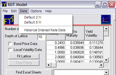
Question 4: How can apply the BDT model to any date over the last 10-years up to current?
A very powerful feature associated with the BDT module is the Historical Interest Rate Data sub menu item:
Selecting Historical Interest Rate Data brings up the following screen:
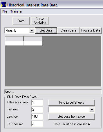
This lets you automatically retrieve historical interest rate data from the Federal Reserve Bank or you can link to your own historical rate file in Excel. We will illustrate the automatic data retrieval. From the drop down menu you can select Monthly, Weekly and Daily. Selecting Monthly retrieves the last ten years of monthly data for the US from the following steps:
i. Click on Get Data
ii. Click on Clean Data
iii. Click on Process Data
iv. Click on Curve Analytics
The following screen now appears:
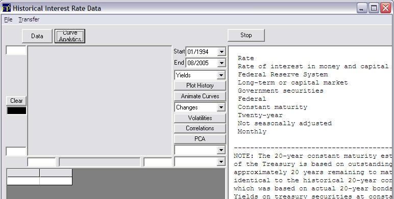
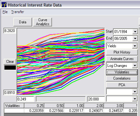
In this example the monthly data from 3-months to 20-years is retrieved from 01/1994 to 08/2005. It is instructive to see how the yield curve has fluctuated over this time. To do so click on Animate Curves:
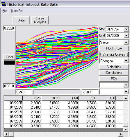
.Observe that the Start Date is 01/1994 and end date is 08/2005. The user can select the start and end date. This fixes the data the sample used to estimate volatility of log changes for the Black Derman Toy model. The spot curve used is the End Date's current yield curve. This is the last row in the above grid beside 08/2005.
Aside: If you want to see the volatility of the log changes. Select Log Changes from the drop down menu and then click on Volatilities. This displays the volatility structure estimated from the historical Yield data from 3-months to 20-years.
Now we are ready to transfer the data to the BDT module. Select Transfer from the above menu:
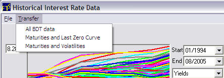
This lets you transfer the desired combination:
All is Maturity, Spot Yield Curve and Volatility Structure
The second selection is Maturity and the Spot Yield Curve associated with the End Date (i.e., 08/2005 in the current example).
Third is Maturity and the Volatility Structure estimated from historical data that in the current example Starts 01/1994 and ends 08/2005.
In this example we will select All BDT Data. The following message pops up:
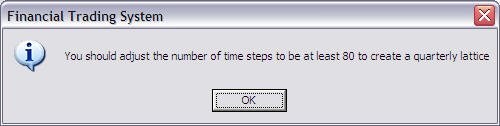
This message refers to the suggested minimum Depth of the Lattice for the BDT module. In this case 80 = 20 years times 4 quarters. You can make the lattice much finer than this if you are using it for valuation purposes but for learning how to use the BDT module 80 is easier to understand. The analogous example is in the original BDT example they provided the date such that the depth of the lattice equal the number of of years.
So following the suggestion above we change the Depth to 80:
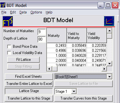
Now by click on Fit Lattice
Find Excel Sheets
Transfer Entire Lattice to Excel
The spreadsheet 1 in Book 5 now contains the BDT risk neutral interest rate tree with a depth of 80 as follows:
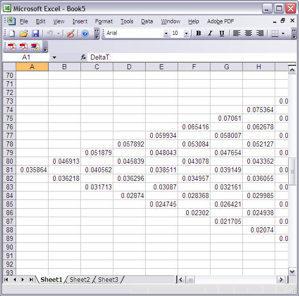
The above is the estimated from the current market data and then lets you repeat the three Questions provided above with respect to the original BDT example. The difference now is that you can apply this to the current spot yield curve/volatility structure.